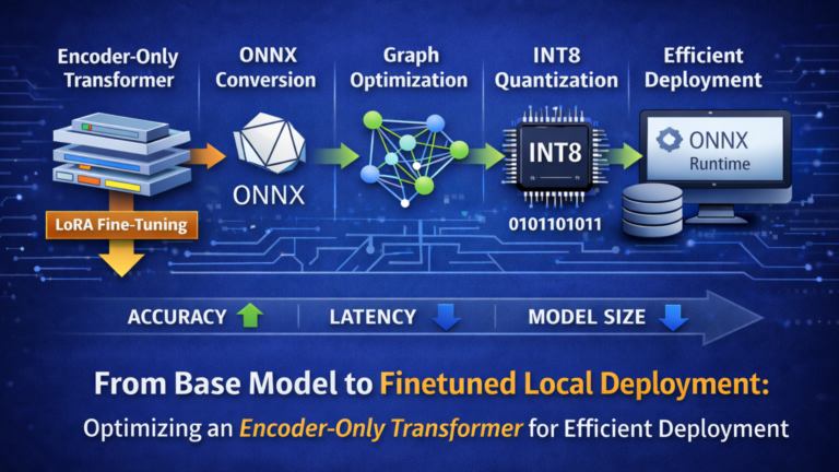
Over the past years, my work has increasingly focused on Artificial Intelligence, particularly the development of AI-powered applications. As my projects evolved, so did my ambition: I wanted Transformer models to run directly on local machines, enabling daily workflows without relying on cloud-hosted environments. Running models locally ensures that private data remains on the device—an essential requirement when handling sensitive information or building systems that demand predictable, low-latency behavior. From both a privacy and architectural perspective, local inference is a meaningful step toward more controlled and self-contained AI systems.

During early experimentation, I worked with tools such as Ollama and AI Studio. While both offer accessible entry points, I eventually transitioned to Microsoft Foundry Local. The decisive advantages were its native ONNX support, integrated fine-tuning workflow, and alignment with production-oriented deployment patterns. This allowed me to establish a coherent end-to-end pipeline—from fine-tuning and model conversion to quantization and fully local execution.

After installing Microsoft Foundry Local and listing available models, you will encounter options like Phi, Mistral, GPT, DeepSeek, Qwen, and their variants. These preconfigured models primarily target chat-oriented workloads and are based on decoder-only, autoregressive Transformer architectures, reflecting the current industry focus on generative systems.

However, my objective was different: I was not building a generative assistant but a high-accuracy classification system. Classification tasks—such as intent detection, sentiment analysis, or structured label assignment—benefit from encoder-only architectures. Unlike decoder-only models, encoder-based Transformers process the entire input bidirectionally, producing stable and context-rich representations that align naturally with discriminative objectives while maintaining predictable inference behavior. For this reason, I deliberately shifted toward an encoder-only Transformer architecture tailored to classification workloads.

Rather than relying on ad-hoc experimentation, I follow a structured AI project lifecycle.

All scripts, configuration files, and evaluation utilities used in this article are available in the accompanying GitHub repository:

👉 Fine-Tuning-and-Deploying-an-Encoder-Only-Transformer

The AI project lifecycle

A production-grade AI project typically follows five structured phases:

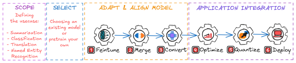
1. Scope – Define the business objective and measurable success criteria.
2. Select – Choose a suitable base model.
3. Adapt & Align – Fine-tune and validate task behavior.
4. Optimize – Convert and optimize for target hardware (e.g., ONNX export, quantization).
5. Integrate – Deploy and operationalize.

Each phase directly influences accuracy, latency, cost, and long-term maintainability. Many production failures occur where optimization and integration were treated as afterthoughts.

Step 1: Scope — define the use case before you touch a model

Before discussing models or hardware, the problem must be defined precisely. Not every workflow requires machine learning, and many so-called AI problems can be solved with deterministic logic. Introducing a model where it is unnecessary adds operational complexity without proportional value.

In this demo, the scoped use case is intentionally focused: email classification as a production workload. Incoming emails—typically up to 256 tokens—must be assigned to one of six operational categories.

	
Categorie
Core Intent




	
forum
Forum posts, discussions, and community notifications


	
promotions
Marketing emails, sales, offers, advertisements.


	
social_media
Notifications from social platforms.


	
spam
Unwanted emails, scams, phishing attempts.


	
updates
System updates, security patches, maintenance notices.


	
verify_code
Authentication codes and verification emails.

The system must operate locally, deliver predictable latency, and remain maintainable without repeated retraining cycles. At the same time, the model must run locally, be callable through APIs, and remain compact enough for efficient inference on local CPU, GPU, or NPU hardware. Most importantly, the workload is strictly classification-oriented rather than generative.

Step 2: Select — choose the right model strategy

Based on the scope requirements, I selected microsoft/deberta-v3-base as the base model. DeBERTa-v3-base provides a strong balance between performance and efficiency: it consists of 12 encoder layers with a hidden size of 768 and approximately 86 million backbone parameters, plus a 128K-token vocabulary that adds about 98 million parameters in the embedding layer, for a total of roughly 184 million parameters. The model builds on the DeBERTa V2 pretraining foundation and was trained on around 160 GB of text data. This profile makes it well suited for high-accuracy classification while remaining practical for fine-tuning and local deployment on a starter-level GPU.

Step 3: Adapt & Align — make the model production-ready

Before processing a base model, Python environments must be defined deliberately. A clear environment strategy is essential for building a stable, reproducible deployment pipeline. A common mistake in AI projects is running the entire lifecycle—from fine-tuning to deployment—within a single environment, which often fails in practice due to dependency conflicts.

Typical issues include mismatched CUDA versions, quantization libraries silently downgrading transformers, or torch upgrades breaking bitsandbytes. Some conversion tools depend on deprecated APIs, and certain packages install successfully but fail at runtime due to binary incompatibilities. Even more problematic are silent failures: a stage completes without errors and produces a seemingly valid artifact, only to fail later during inference or conversion. To mitigate this, each artifact should be validated immediately after every stage.

The most reliable solution is to separate responsibilities into dedicated Python environments. I created three environments:

• .venv_finetune for training and validation
• .venv_onnx for merging, conversion, and optimization
• .venv_quantize for quantization

This separation establishes clean dependency boundaries, improves reproducibility, and reflects a production-ready engineering approach.

1. Create .venv_finetune

py -3.10 -m venv .venv_feintune  # create a new environment
.\.venv_feintune\Scripts\activate  # activate the environment
python -m pip install --upgrade pip  # upgrade pip

Then check the CUDA version:

nvidia-smi

Example output:

+-----------------------------------------------------------------------------------------+
| NVIDIA-SMI 573.92                 Driver Version: 573.92         CUDA Version: 12.8     |
|-----------------------------------------+------------------------+----------------------+

Based on this output, install the matching PyTorch build, then install PyTorch with CUDA:

pip install torch torchvision torchaudio --index-url https://download.pytorch.org/whl/cu128

Note: NVIDIA drivers must already be installed on your system.

If you want to use CPU-only training (not recommended due to significantly longer training times), install:

pip install "torch>=2.6.0" torchvision torchaudio

Then install the remaining dependencies:

pip install -r requirements_finetune.txt

Finally verify CUDA availability:

python -c "import torch; print('CUDA available:', torch.cuda.is_available()); print('GPU:', torch.cuda.get_device_name(0) if torch.cuda.is_available() else 'None')"

2. Create .venv_onnx

Deactivate the fine-tuning environment first:

deactivate # deactivate the current environment

Then create and configure the ONNX environment:

py -3.10 -m venv .venv_onnx 
.\.venv_onnx\Scripts\activate    
python -m pip install --upgrade pip 
pip install -r requirements_onnx.txt

3. Create .venv_quantize

Deactivate the ONNX environment first:

deactivate

Then create and configure the quantization environment

py -3.10 -m venv .venv_quantize
.\.venv_quantize\Scripts\activate
python -m pip install --upgrade pip
pip install -r requirements_quantize.txt

Preparing the dataset

For fine-tuning, the dataset is divided into three disjoint subsets: training, validation (evaluation), and test.

Each serves a distinct purpose. The training set is used to update the model’s weights during fine-tuning and therefore cannot be used to measure real-world performance. The validation set is used during training to monitor generalization, tune hyperparameters, and select the best checkpoint; since training decisions are based on validation performance, it cannot serve as the final benchmark. The test set is kept completely separate until training is finished and is used only once to evaluate the final model; if it influences training decisions, it effectively becomes another validation set and loses its statistical meaning.

Dataset selection

For this project, I use the jason23322/high-accuracy-email-classifier dataset available on Hugging Face. It contains more than 12,000 labeled emails across six categories and is specifically designed for high-accuracy email classification. When fine-tuned properly, models trained on this dataset can achieve accuracy above 98%, making it a realistic and suitable choice for this demonstration.

From the dataset repository, the following files are required:

1. train.json
2. test.json

Dataset transformation

Before fine-tuning with microsoft/deberta-v3-base, the dataset must be converted into the expected input format. The original dataset contains multiple fields:

[
  {
    "id": "...",
    "subject": "...",
    "body": "...",
    "text": "...",
    "category": "...",
    "category_id": 2
  }
]

For sequence classification of microsoft/deberta-v3-base , only two fields are required:

1. text → input sequence
2. label → numerical class ID

The dataset is therefore must be transformed into the following structure:

[
  {
    "text": "...",
    "label": 2
  }
]

This ensures compatibility with the model’s classification head and enables seamless integration into the fine-tuning pipeline.

Creating train / eval / test subsets

To prepare the final datasets, the script create_data_subsets.py located in scripts/data performs two tasks:

1. Splits the original test.json into:
   • eval_dataset.json
   • test_dataset.json
2. Converts all files into the required {text, label} format.

Run:

python .\scripts\data\create_data_subsets.py 
  -itr .\data\raw\train.json 
  -ite .\data\raw\test.json 
  -o .\data\data-subsets

After execution, the final dataset-structure within the data directory is organized as follows:

📁 data
├── 📁 data-subsets
│   ├── 📄 eval_dataset.json
│   ├── 📄 test_dataset.json
│   └── 📄 train_dataset.json
└── 📁 raw
    ├── 📄 test.json
    └── 📄 train.json

Fine-tuning the base model with LoRA

To fine-tune microsoft/deberta-v3-base, access to the model repository on Hugging Face is required. First, create a personal access token in your Hugging Face account settings, then authenticate your local environment using the Hugging Face CLI:

hf auth login

Once authenticated, start the fine-tuning process with:

python .\scripts\finetune_lora_deberta.py 
  --model microsoft/deberta-v3-base 
  --train_file .\data\data-subsets\train_dataset.json 
  --eval_file .\data\data-subsets\eval_dataset.json 
  --output_dir .\models\1_LoRA-adapter 
  --max_length 256 
  --epochs 5 
  --per_device_train_batch_size 8 
  --gradient_accumulation_steps 4 
  --lr 2e-4 
  --warmup_steps 336 
  --weight_decay 0.01 
  --lora_r 16 
  --lora_alpha 32 
  --bf16

After training completes, you will see output similar to:

trainable params: 2,683,398 || all params: 187,110,156 || trainable%: 1.4341
...
{'eval_loss': '0.04417', 'eval_accuracy': '0.9948', 'eval_f1_macro': '0.9948', ...}
...
Saved LoRA adapter + tokenizer to: .\models\1_LoRA-adapter

Only about 1.43% of the model’s parameters are updated during training, which is the key advantage of LoRA (Low-Rank Adaptation): it adds small trainable matrices on top of a frozen base model, significantly reducing memory consumption and training time while preserving strong performance. After five epochs, the model achieves

• Accuracy: 99.48%
• Macro F1-score: 0.9948
• Eval loss: 0.044

These results indicate excellent classification performance and strong generalization on the validation set. The trained LoRA adapter and tokenizer are stored in models\1_LoRA-adapter

Step 4: Merge, convert, optimize, quantize

Fine-tuning with LoRA produces an adapter, not a standalone model. The adapter contains only the low-rank weight updates and must be combined with the base model before deployment. The next steps are therefore:

1. Evaluate the LoRA adapter.
2. Merge the adapter into the base model.
3. Convert the merged model to ONNX.
4. Optimize the ONNX graph using Olive.
5. Quantize the model for further performance gains.

4.1 Evaluating the LoRA adapter

Before merging, I evaluate the adapter together with the base model on a subset of 200 unseen test samples:

python .\scripts\eval\evaluate_LoRA_adapter.py 
  --base microsoft/deberta-v3-base 
  --adapter .\models\1_LoRA-adapter 
  --testdatapath .\data\data-subsets\test_dataset.json
  --testcount 200

Output:

Testing sample 200/200...
Accuracy with unmerged adapter: 99.50%

An accuracy of 99.50% confirms that the adapter generalizes well and that the fine-tuning configuration is stable.

4.2 Merging LoRA into the base model

The merge step combines the base model with the fine-tuned LoRA weights to produce a single, self-contained artifact. This simplifies downstream conversion, optimization, and deployment; skipping this step would complicate runtime handling and ONNX export.

python .\scripts\eval\merge_deberta_ONNX.py 
  --base microsoft/deberta-v3-base 
  --adapter .\\models\1_LoRA-adapter 
  --output .\models\2_merged_model

Output:

✓ Fine-tuned model loaded.
✓ Model has 6 labels
🔄 Merging LoRA adapter into base weights...
✅ Adapter merged successfully
...
✅ Merged model saved to: .\models\2_merged_model
...
✅ Tokenizer saved to: .\models\2_merged_model

This script loads the fine-tuned checkpoint, applies the LoRA adapter, merges the adapter weights into the base model, ensures correct label mappings, and saves the merged model and tokenizer into models/2_merged_model. At this stage, the model is fully self-contained and ready for conversion to ONNX.

4.3 Converting to ONNX with Olive

Next, the merged Hugging Face model is converted into ONNX format using Microsoft Olive. For a detailed introduction to Olive and its role in deployment pipelines, see my dedicated guide about Olive, ONNX and ONNX Runtime in the blog.

Activate the ONNX environment:

deactivate # deactivate the current environment
.\.venv_onnx\Scripts\activate # activate the environment

Then convert the mode to ONNX format:

olive capture-onnx-graph 
  --model_name_or_path .\models\2_merged_model
  --task text-classification 
  --output_path .\models\3_converted_onnx

Olive performs an ONNX Runtime–aware export using optimized backend paths, preparing the model for efficient execution under ONNX Runtime. A poorly executed export can introduce numerical inconsistencies, performance regressions, operator incompatibilities, or cross-environment inference differences. Using Olive helps ensure a stable and deployment-ready ONNX graph. The converted model is saved under models/3_converted_onnx.​

To verify correctness and ensure no accuracy degradation occurred during conversion, evaluate the ONNX model:

python .\scripts\eval\model_evaluation.py 
  --model .\models\3_converted_onnx 
  --testdatapath .\data\data-subsets\test_dataset.json 
  --testcount 200

This validation step confirms that the exported ONNX model produces consistent predictions compared to the original PyTorch model.

4.4 Optimizing the ONNX model with Olive

After conversion, the next step is to apply ONNX Runtime transformer optimizations using Olive. These optimizations improve inference efficiency by restructuring and simplifying the computational graph.

A minimal configuration:

{
  "input_model": {
    "type": "ONNXModel",
    "model_path": "models/3_converted_onnx/model.onnx"
  },
  "passes": {
    "optimize": {
      "type": "OrtTransformersOptimization",
      "config": {
        "model_type": "bert",
        "opt_level": 2
      }
    }
  },
  "engine": {
    "output_dir": "models/4_optimized"
  }
}

Run:

olive run --config .\olive-configs\optimize_config.json

This optimization pass performs several graph-level improvements, including operator fusion, constant folding, redundant node elimination, and transformer-specific optimizations such as attention and layer normalization fusion. It also prepares the model for downstream quantization. For DeBERTa, using model_type: “bert” with opt_level: 2 provides a practical balance: it enables advanced transformer optimizations without applying the most aggressive transformations and in practice can yield noticeable inference speedups while preserving numerical stability and accuracy. The optimized model is stored in models/4_optimized.

Olive supports following optimization levels:

	
opt_level
Description




	
0
No optimization


	
1
Basic graph optimizations (constant folding, redundant node removal)


	
2
Extended transformer optimizations (attention fusion, GELU approximation, layer norm fusion)


	
99
Maximum optimization (most aggressive; may affect numerical precision)

4.5 Quantization — making the model edge‑friendly

To further improve performance—particularly on CPU and edge devices—I apply dynamic INT8 quantization. This reduces model size and improves inference latency without requiring calibration data.

Deactivate the ONNX environment and activate the quantization environment:

deactivate  # deactivate the current environment
.\.venv_quantize\Scripts\activate # activate the environment

Then run:

olive auto-opt 
  --model_name_or_path .\models\4_optimized 
  --device cpu 
  --provider CPUExecutionProvider 
  --output_path .\models\5_quantized 
  --log_level 1 
  --task text-classification

This step applies dynamic INT8 quantization. It converts FP32 weights in linear layers and embeddings to INT8, while activations are quantized dynamically at inference time. Numerically sensitive operations—such as attention and layer normalization—remain in floating point to preserve stability. Because quantization parameters are computed on the fly, no calibration dataset is required.

For classification workloads, INT8 dynamic quantization often reduces model size by up to 4× and significantly improves CPU inference speed, with minimal impact on accuracy. The quantized model is saved in models/5_quantized and is ready for deployment.

At this point, the project includes a fine-tuned and merged DeBERTa classifier, converted to ONNX, optimized for transformer inference, and compressed for efficient local execution.

📁 models
├── 📁 1_LoRA-adapter
├── 📁 2_merged_model
├── 📁 3_converted_onnx
├── 📁 4_optimized
└── 📁 5_quantized

Each subdirectory represents a distinct stage in the model lifecycle—from the initial LoRA adapter generated during fine-tuning to the fully optimized and quantized deployment artifact. This structured organization ensures clear separation between transformation steps and supports reproducibility, traceability, and maintainability throughout the pipeline.

Step 5: Deploy — run where it actually matters

With optimization complete, the final step is deployment. My original objective was to deploy the fine-tuned model using ONNX Runtime within Microsoft Foundry Local. However, during integration testing, the model failed to execute as expected.

Further investigation revealed the reason: Microsoft Foundry Local is designed for text generation workloads based on decoder-style large language models such as LLaMA, GPT, Phi, and Mistral. It relies on onnxruntime-genai, which implements token-by-token generation loops, KV-cache handling, and sampling strategies. DeBERTa, by contrast, is an encoder-only model. It performs classification in a single forward pass and does not rely on autoregressive generation mechanisms. Because Foundry Local is built specifically around generation-oriented runtimes, encoder-based classification models are currently outside its intended scope.

As a result, while the ONNX model is fully optimized and production-ready, it must be deployed using standard ONNX Runtime inference pipelines—either as a local service or embedded application—rather than the Foundry Local generation framework.

Using ONNX Runtime directly

The simplest and most portable way to deploy this classifier is to load the ONNX model with standard ONNX Runtime in a local service or application. Here is a minimal Python example:

import onnxruntime as ort
from transformers import AutoTokenizer
import numpy as np

MODEL = "models/4_optimized/model.onnx"
TOKENIZER = "models/4_optimized"
ID2LABEL = {
    0: "forum",
    1: "promotions",
    2: "social_media",
    3: "spam",
    4: "updates",
    5: "verify_code",
}

session = ort.InferenceSession(MODEL, providers=["CPUExecutionProvider"])
tokenizer = AutoTokenizer.from_pretrained(TOKENIZER)

def classify(text: str) -> str:
    inputs = tokenizer(text, return_tensors="np", truncation=True, max_length=256)
    logits = session.run(
        None,
        {
            "input_ids": inputs["input_ids"].astype(np.int64),
            "attention_mask": inputs["attention_mask"].astype(np.int64),
        },
    )[0][0]
    pred_id = int(np.argmax(logits))
    return ID2LABEL[pred_id]

print(classify("Your verification code is 123456"))
print(classify("70% off sale today only!"))

python .\usage\simple_client\app.py

Output:

verify_code
promotions

Performance impact of each optimization stage

The chart below presents a comparative analysis of the base, fine-tuned, ONNX-converted, optimized, and quantized model variants across four key metrics: accuracy, F1 score, inference time, and model size. All measurements were conducted using the complete test set of 1,351 samples, with the full dataset consistently applied at each stage to ensure a fair and reliable evaluation.

Fine-tuning is the primary driver of predictive performance: the base model achieves only 14.06% accuracy and 9% F1, while the fine-tuned model reaches roughly 99.5% on both metrics. ONNX conversion and transformer optimization preserve this performance, demonstrating that export and graph-level improvements do not degrade model quality. Quantization maintains accuracy at 99.56%, confirming that INT8 dynamic quantization has no meaningful impact on classification results for this workload.

Inference latency improves progressively from roughly 456 ms (fine-tuned) to 413 ms (optimized), with the largest gain achieved through quantization at approximately 306 ms. Model size remains near 704 MB until quantization reduces it to 213 MB—about a 70% reduction—making the classifier far more suitable for local and edge deployment.

Overall, fine-tuning determines accuracy, while conversion, optimization, and quantization systematically improve deployment efficiency without sacrificing predictive performance.

Final toughts

This project started with a simple idea—run Transformer models locally—and evolved into a fully engineered pipeline for high-accuracy email classification. By deliberately choosing an encoder-only architecture, fine‑tuning it with LoRA, and then moving through ONNX conversion, graph optimization, and INT8 quantization, the final quantized model achieves over 99.5% accuracy on the test set while remaining compact and fast enough for everyday local use.

In practice, the journey also highlighted how fragile AI tooling can be: overlapping CUDA, PyTorch, and optimization dependencies make it unrealistic to rely on a single “magic” toolchain. A mixed approach—combining the dedicated Olive CLI commands and also per json configured olive run workflows with Python processing—proved more robust, because it allowed each stage to use the most stable library stack while still benefiting from Olive’s hardware‑aware optimization passes and automation. Paired with clear environment boundaries, explicit validation after each step, and a deployment strategy built on standard ONNX Runtime, this hybrid setup shows how you can turn a research‑grade model into a resilient, edge‑friendly AI component without sacrificing maintainability or control.

References

Dataset: High Accuracy Email Classifier, available at Hugging Face (jason23322).
Model: deberta-v3-base

Onnx Runtime

Olive CLI Reference